Tutorial Overview

This tutorial demonstrates some simple spatial overlay analysis of polygon data using the IDEAS data model, as described in Robertson et al. 2020.

Preliminaries

We will load some sample data from the stampr package, and pull out two polygons to demonstrate overlay operations.

library(stampr)
library(sp)
data(mpb)
P1 <- subset(mpb, TGROUP==1)[5,]
P2 <- subset(mpb, TGROUP==2)[7,]
plot(P2, border="green")
plot(P1, add=TRUE, border="blue")

First we need to load some libraries;

library("dplyr")
library("dbplyr")
library("DBI")
library("leaflet")
library("sf")
library("RODBC")
library("nzdggs")

Loading Polygon Data from IDEAS

We will use the con data connection to access a table called mpb which has the same data from the stampr package in IDEAS format.

mpb.i <- tbl(con,"MPB")
grid <- tbl(con,"FINALGRID2") %>% filter(RESOLUTION==19)
head(mpb.i)
#> # Source:   lazy query [?? x 4]
#> # Database: NetezzaConnection
#>        DGGID VALUE KEY        TID
#>        <dbl> <int> <chr>    <int>
#> 1 4921587640     1 BOUNDARY  1264
#> 2 4921646690     1 BOUNDARY  1264
#> 3 4921587640     0 ID        1264
#> 4 4921646690     0 ID        1264
#> 5 4921587640  1264 tid       1264
#> 6 4921646690  1264 tid       1264

We want to pull out those same two polygons by identifying them by their ID values, as follows:

ID1 <- P1$ID
ID2 <- P2$ID

P1.i <- mpb.i %>% filter(KEY=="ID") %>% filter(VALUE==ID1) %>% inner_join(., grid, "DGGID") %>% mutate(WKT=inza..ST_AsText(GEOM)) %>% collect()
P2.i <- mpb.i %>% filter(KEY=="ID") %>% filter(VALUE==ID2) %>% inner_join(., grid, "DGGID") %>% mutate(WKT=inza..ST_AsText(GEOM)) %>% collect() 

dbDisconnect(con)

plot(st_as_sf(P2.i, wkt='WKT', crs = 4326)['TID'], col='green', reset=FALSE)
plot(st_as_sf(P1.i, wkt='WKT', crs = 4326)['TID'], add=TRUE, col='blue')

Overlay Analysis using IDEAS data model

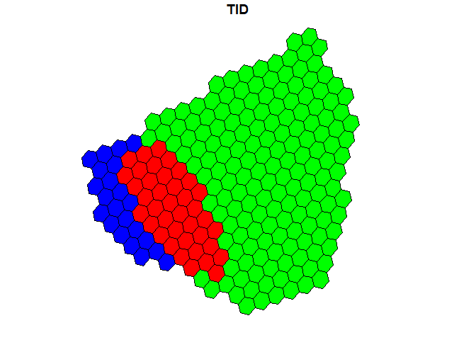
Intersection

intersection <- P1.i %>% inner_join(., P2.i, "DGGID")
plot(st_as_sf(P2.i, wkt='WKT', crs = 4326)['TID'], col='green', reset=FALSE)
plot(st_as_sf(P1.i, wkt='WKT', crs = 4326)['TID'], add=TRUE, col='blue')
plot(st_as_sf(intersection, wkt='WKT.x', crs = 4326)['TID.x'], add=TRUE, col='red')

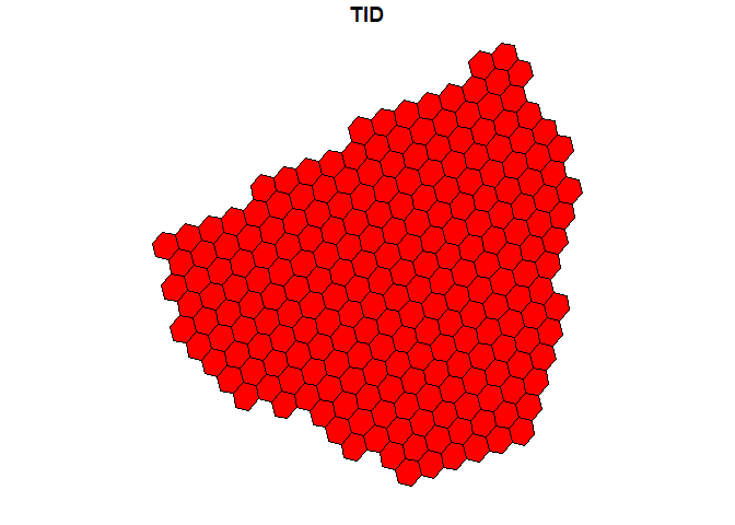
Union

union <- union_all(P1.i, P2.i) %>% distinct(DGGID, .keep_all = TRUE)
plot(st_as_sf(union, wkt=c('WKT'), crs = 4326)['TID'], col='red')

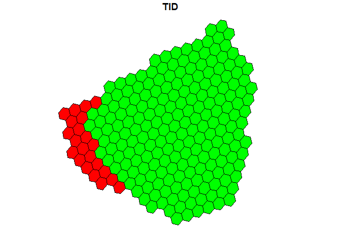
A NOT B

ANotB <- P1.i %>% anti_join(., P2.i, "DGGID")
plot(st_as_sf(P2.i, wkt='WKT', crs = 4326)['TID'], col='green', reset=FALSE)
plot(st_as_sf(ANotB, wkt=c('WKT'), crs = 4326)['TID'], add=TRUE, col='red')